
Guidance on incorporating economic use information into Marine Protected Area network design
Economic Policy and Research
Economic Analysis and Statistics Directorate
Strategic Policy Sector
July 2017
Foreword
To support MPA network development, Economic Analysis and Statistics (EAS, Strategic Policy Sector, DFO) was tasked to develop guidance on incorporating spatial socio-economic (SE) data into MPA network design processes, including discussion of: the purpose and limitations of SE data in this context; the scope and types of SE data to be used; options and recommendations for how to combine data for multiple uses in the network design analysis; and where national consistency will be important or required. The guidance was developed for regional practitioners working on bioregional MPA network planning.
The guidance was developed by EAS with input from Oceans staff in NHQ and all regions, and from DFO economists in all regions, and in consultation with other departments, including Natural Resources Canada, Parks Canada and Environment and Climate Change Canada.
The aim of this document is to provide guidance that is general and flexible enough to be used in all bioregions, while being specific enough to provide for some level of national consistency. In the 5 priority bioregions where network development is already proceeding, there is a wide range of different approaches to network design. While some parts of this guidance are presented in a very technical way, the underlying concepts that drive the technical recommendations should in most cases be transferrable to less technical approaches.
Table of contents
- Foreword
- Table of contents
- 1 Background and scope
- 2 Guidance
1 Background and scope
This section describes the general context in which this guidance is being provided, and establishes the intent and scope of the guidance. It first briefly describes the MPA network development process as laid out in the National Framework for Canada’s Network of Marine Protected AreasFootnote 1 (hereafter the MPA Network Framework). It then lays out the purposes and limitations of SE data and analysis in this process, and the subset of these purposes for which the current guidance is provided. Links to other guidance documents are highlighted, especially the Framework for Integrating Socio-Economic Analysis in the Marine Protected Areas Designation ProcessFootnote 2 (hereafter the MPA SE Framework). Finally, the role of interested parties in the process is described and expectations about national consistency are addressed.
1.1 MPA network development process
The MPA Network Framework lays out the purpose and context of designing and establishing bioregional networks of MPAs. It would be helpful for readers of the current guidance, especially those new to the MPA network process, to review the entire Framework, but some particularly important components in the context of the current guidance include:
- Section 3 on the network’s goals, including National Network Goal Two which has the strongest socio-economic component. This goal is “to support the conservation and management of Canada's living marine resources and their habitats, and the socio-economic values and ecosystem services they provide.” Note that Goal Two, along with Goal Three, is considered a secondary goal of the national network. Goal One, which is concerned primarily with biodiversity conservation, is considered the primary goal;
- Section 6, which explains that the MPA network will be planned using the spatial framework of 13 ecologically defined bioregions in Canada’s oceans and Great Lakes;
- Section 8 on guiding principles for the development of the network, especially principle 4, which is “Take socio-economic considerations into account. Once the ecological conservation needs have been identified, consider socio-economic information to achieve an optimal, cost-effective network design and also to plan individual new network MPAs.” We refer to this principle as the cost-effectiveness principle.
- Section 10.2 on the network development process. This section has since been superseded (see below), but still provides useful details on some aspects of the process. In particular, step 5 in that process says that in network design we will “seek to understand and minimize potential economic and social consequences.”
The most current description of the network development process is in Figure 1, which outlines 4 elements: (1) data and information gathering; (2) MPA network design; (3) implementation; (4) and management and monitoring. This process is to be applied at the bioregional level to design each bioregional network.
The dotted rectangles in the diagram highlight the areas where SE data and analysis will (or may) play a role in network development processes. More detail is provided in the next section on these roles, and which subset is addressed in this guidance document.
Figure 1. Four elements of bioregional MPA network development (Provided by NHQ Oceans)
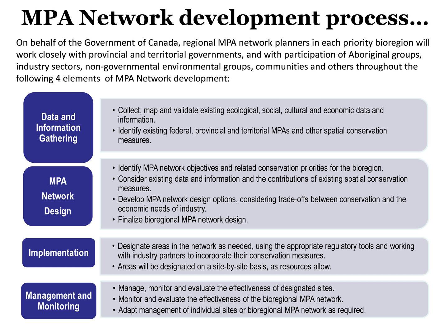
Figure 1 - Text equivalent
Step 1 is data and information gathering which includes collecting, mapping and validating existing ecological and economic data and information, and identifying existing conservation measures.
Once that work is completed, the MPA network is designed in step 2. This work involves identifying MPA network objectives and conservation priorities for the bioregion, considering the data and information for existing conservation measures, developing MPA network design options (having considered trade-offs between conservation and economic needs), and finalizing the bioregional network design.
Step 3 is implementation, where marine protected areas and other conservation measures are designated using appropriate regulatory tools, and in consideration of available conservation measures used by industry partners.
Step 4 is management, as well as monitoring to evaluate the effectiveness of the designated sites and the network as a whole. Management measures are adapted as required.
Socio-economic data and analysis play a role in all four steps of the MPA network development process.
1.2 Purpose and limitations of SE data in network development
Following the 4 elements outlined in Figure 1, there are several places in the bioregional network development process where SE data and analysis can (or may) play a role.
- The first element (data and information gathering) includes the collection of SE data, whether already available or to be newly collected specifically for the network process. This element is addressed in the current guidance.
- In the second element (MPA network design), SE data will be used to apply the cost-effectiveness principle outlined in the MPA Network Framework, as one aspect of sub-element 3, “Develop MPA network design options….” This is the primary focus of the current guidance document. SE data and analysis may also be used in 2 other parts of element 2: (1) before developing network design options, SE data may be used in sub-element 1 to inform bioregional MPA network objectives related to National Network Goal TwoFootnote 3. Guidance on this use of SE information has been developed separatelyFootnote 4; and (2) once a set of network design optionsFootnote 5 is developed, discussions with interested parties about these options will likely be informed by general SE informationFootnote 6 about each option, as part of a process to finalize the MPA network design (sub-element 4). Guidance with respect to this use of SE information is not included here, but may be developed at a later date.
- In the third element (implementation), SE information and analysis will be used in the creation of MPA network action plansFootnote 7 and subsequent site designation processes. In the case of Oceans Act (OA) MPAs, site designation will be done as outlined in the MPA SE Framework, while in the case of other legal instruments (e.g., National Marine Conservation Areas (NMCAs)) the SE data and analysis will be compiled and analyzed in keeping with the relevant practices for those legal instruments. Thus, this use of SE information is not addressed in this document.
- There may be a role for SE data in the fourth phase, managing and monitoring MPA sites and the bioregional networks. However, this use is also beyond the scope of the current guidance.
The core focus of this document, then, is to address the processing of spatial socio-economic data, and the incorporation of these data into the second element of the network design process, more specifically the third sub-element, “develop MPA network design options,” which we will refer to as the network design analysisFootnote 8. The analytical framework implied by the MPA Network Framework is that the analysis will “minimize potential economic and social consequences,” subject to the constraint that network objectives are met.
It is worth briefly exploring what is meant by each of the key terms in this analytical objective, as this will help establish the scope of the guidance document and of the analyses to be conducted.
Minimize: Minimization in the context of the network design analysis must be understood together with the other side of the analytical question, i.e., that network objectives be met. In other words, it can be thought of in “all else being equal” terms, so that if there are many potential network designs that would attain network objectives, the network design option that should be selected is the one that minimizes potential negative economic and social consequences. However, the analytical approach taken will likely not be a strict or exact minimization, but rather an approximate or near-minimization: the analytical requirements to obtain an exact minimization are too great given available data and tools, and discussion with interested parties and partners will likely require some deviation from the hypothetical exact minimum.
Potential: There are 2 aspects of this term when discussing “potential” impacts on economic activities:
- Is the activity under consideration currently taking place in the area in question, and/or may the activity take place at some point in the future?; and
- Assuming that the activity occurs (or will likely occur) in the area, will there in fact be consequences for that activity arising from the management measures that are ultimately implemented?
The second aspect is addressed below in the discussion of “consequences.” For the first aspect, related to possible future activities, it is appropriate to align the approach in network design with that in the MPA SE Framework, as follows. Possible future activities should only be included in the analysis if there is some formal commitment to allow these activities in the near future (i.e., within the next 10 years). This would include activities for which a clear intent to undertake the activity (e.g. business plans, permits, submission of plans for approvals, etc.) can be established. The inclusion of such activities in the analysis should be based on evidence which supports an assertion of imminent economic growth. For example, for the oil and gas sectorFootnote 9 the potential presence of oil or gas resources based on seismic surveys would not be sufficient to include the activity in the analysis. Similarly, for fisheries, there should be reasonably strong evidence that significant future catches are probable in areas under consideration for the network.
Economic and Social: The Treasury Board Secretariat’s cost-benefit analysis guide uses the term “economic” to refer to matters that “affect economic welfare and economic growth,” and the term “social” to refer to “distributional impacts of policies,” i.e., how the costs and benefits of a policy are distributed among interested parties. We will follow this approach, also adopted in the MPA SE Framework, in this guidance document. While there may be other elements of “social consequences” that may be of interest, it is beyond the expertise of EAS to provide guidance on these.
Consequences: With a few exceptions, an MPA network will have both positive and negative consequences for most of those who use marine ecosystems (e.g., see the benefits and costs listed in section 7 of the MPA Network Framework). In theory, the network design analysis could include both the benefits and costs of the network for each group of users; in other words, the analysis could follow a benefit-cost analysis (BCA) framework along the lines of that outlined in the MPA SE Framework. However, given the spatial scale of the bioregions this would impose a very heavy data and analytical burden. Furthermore, while a BCA is a regulatory requirement for OA MPA designation, there is no such requirement at the network design stage.
Therefore, this guidance document focuses on assessing the extent to which different economic uses overlap with network design options, which in turn is used as an indication of the extent to which a given design may impose opportunity costsFootnote 10 on users by limiting their activities in some areas. Assessments of opportunity costs will be highly uncertain at this stage of the network design process because:
- The management measures to be applied in each site will not yet be specified, so it is impossible to know for certain the extent to which any given activity will be impacted by the network. For example, areas selected for inclusion in the network may end up being designated as an Oceans Act MPA, a NMCA, a fisheries closure, etc., and within these different legal instruments a range of specific management measures might be specified that may or may not affect a given sector; and
- Some activities might be able to relocate with minimal costs and with little effect on other users in the new location, meaning that the actual cost imposed by the network will be lower than that estimated by the overlap approach (which effectively assumes that activities with which the network overlaps will cease once the network is implemented). However, it will be difficult to estimate these costs and relative mobility of economic sectors in such a large-scale analysis, let alone the impacts on users of the areas to which the displaced sectors move. It will be more feasible to address these dynamic issues during network implementationFootnote 11.
Recognizing these uncertainties, as well as the data and analytical limitations noted above, the approach recommended in this guidance is to assess the relative importance of each planning unitFootnote 12 in the bioregion to each economic use whose activities are expected to be affected by the network. Relative importance will then be used as a proxy for the opportunity costs that may be imposed on each economic use should the planning unit under consideration be identified for inclusion in the network. The bulk of the guidance focuses on how to assess “relative importance” for each economic use, and how to combine these assessments for multiple economic uses into a single network design analysis.
1.3 Link to the Oceans Act MPA Socio-economic Framework
It is important to recognize that MPA network design occurs at an earlier stage of the network development process than the OA MPA designation process. Network design is element 2 of Figure 1. Element three of network development can eventually lead to the designation of an area(s) as, for example, an OA MPA, a NMCA under the Canada National Marine Conservation Areas Act, or another legal instrument (e.g., a fisheries closure), depending on the measures required to attain the site-specific conservation objectives associated with that areaFootnote 13. For areas that are to be designated as OA MPAs, the MPA network development process is the basis for the identification of Areas of Interest (AOIs), which will ultimately be put forward for OA MPA designation. See the MPA SE Framework (especially Figures 1 and 3) for a description of how the designation process then continues, and the role of SE information in that process.
1.4 Engagement of interested parties in the network design analysis
As should be clear from the MPA Network Framework, engagement of interested parties is a fundamental principle and will occur throughout MPA network development and implementation. When engagement is undertaken with respect to the issues dealt with in this guidance, it should be conducted in a way that is consistent with national direction on MPA network engagement and any bioregional network-specific engagement strategies.
The work described in this guidance document that is most likely to benefit from discussion with economic users is that concerning the representation of sectors in the analysis (i.e., section 2.2.2). As explained above, the purpose of the analysis is to reflect the relative importance of different planning units to each economic use. People participating in that sector are likely to be among the best equipped to inform discussions about how this importance should be reflected, including around issues of spatial distribution of catch/value, etc., and especially in sectors where data are sparse or completely unavailable. This engagement might contribute to generating the maps to be used, but can also be used to validate maps generated from internal data, or through combining internal data and the results of engagement.
1.5 National consistency
The guidance in this document provides for flexibility in some areas, but also provides a basis for national consistency in many aspects of integrating SE data into MPA network design. More specifically:
- The application of SE data should be consistent with the purpose, limitations and scope outlined in section 1.2Footnote 14.
- The specific approaches and recommendations provided in section 2 are key and should be adopted whenever possible as they allow for national consistency in the analysis.
The general expectation is that regions will work in keeping with the guidance provided here, as well as with further revisions of the guidance. In some cases, departures from the guidance might be appropriate or even unavoidable. For example, this might occur in cases where work has already been completed in a bioregion before the guidance was completed, or where the guidance is revised after the completion of some of the work. If such departures from this guidance are being contemplated:
- The reasons for the proposed departures from the guidance should be clearly documented; and
- They should be discussed with NHQ Oceans and/or EAS to assess whether or not such departures might have implications in other regions and/or at the national level.
2 Guidance
This section is the core of the guidance for how to prepare and use SE data in the network design analysis. It first outlines options for the type of network design analysis that might be undertaken. It then addresses 3 major analytical steps that must be addressed to incorporate SE data: deciding which sectors to include in the analysis; how to represent individual sectors in the analysis; and how to combine multiple sectors into a single, coherent analysis.
2.1 Types of analysis
Recall that the analysis under discussion aims to identify a set of planning units (PUs; where each PU is a polygon or grid cell on a map) that, if included in the MPA network, would minimize negative “potential economic and social consequences” while meeting a set of network objectives. In practice, this means that the analysis will seek a network design that meets the network’s objectives while, to the extent possible, minimizing overlap with areas of importance to the economic sectors included in the analysis. A wide range of analytical approaches could be taken in this analysis; this section outlines the range of options in terms of: qualitative versus quantitative analyses; the options available within quantitative analyses; possible combinations of these types of analyses; and other issues and considerations.
2.1.1 Qualitative versus software-based analysis
One important distinction between types of analyses is the extent to which they rely on qualitative/expert consideration of spatial biological and SE data, versus the use of these data in quantitative software.
2.1.1.A Qualitative map/overlap analysis
One example of a “qualitative” approach would be to map ecological data (e.g., ecologically and biologically significant areas), and then examine these data together with economic data, in consultation with interested parties. These maps could be explored with the objective of identifying areas for inclusion in the network based on (a) overlap with areas containing conservation priorities and (b) lack of overlap with important areas for economic uses. This method could be conducted by DFO staff, or in consultation with other experts in a Delphic approach (i.e., by surveying experts regarding important areas to include in the network), and would not generally include the use of decision-support software. However, this approach would likely make use of some specialized software, such as a geographic information system (GIS), to process the required spatial data.
This approach has the advantage of being flexible, and removes the requirement to put data sets from a range of economic sectors into a single, comparable quantitative format. On the other hand, this method is not reproducible (i.e., it would likely give very different results if redone at a different time or with different staff or experts), offers relatively little transparency about how a specific design was arrived at, and is therefore more subjective than methods using decision-support software. It is also more difficult to incorporate large amounts of data with this approach.
2.1.1.B Software-based analysis
This approach involves the use of decision-support software to integrate biological and SE data and propose network design options. Such software has the capability to incorporate very large amounts of biological and SE data and to consider many different network configurations in an attempt to find a cost-effective network configuration, making it useful for the complicated and large-scale analyses required in many Canadian bioregions.
These software-based approaches have the advantage of being relatively reproducible and relatively transparent (e.g., with the documentation of input parameters), but will tend to have higher data and technical requirements than qualitative approaches. It is important to remember when considering this type of software that they provide decision support only, that is, they provide design options that should be reviewed in detail, discussed with interested parties, and adjusted where appropriate until a satisfactory design option (or options) is arrived at. Note also that calling this approach “software-based” does not imply that computer software will not be used in more qualitative approaches, but that some type of optimization algorithm in the software is the primary means by which a cost-effective network design option is identified.
2.1.1.C Hybrid approaches
In some situations it may be appropriate to combine elements of the qualitative and software-based approaches. For example, if high-quality, high-resolution data are available for some economic uses but only low-resolution data are available for others, it may be appropriate to (1) conduct a software-based analysis for sectors where data are available, and then (2) overlay available information on other sectors with the output of the initial software-based analysis, and use more qualitative approaches to account for the additional sectors. Such hybrid approaches may be able to use the advantages of both the software-based and qualitative methods, depending on the specific circumstances in a particular bioregion.
Recommendation: Software-based analyses are recommended, but qualitative/ overlap-based and hybrid analyses are also acceptable where regional staff deem that they are more appropriate, especially in cases of limited data availability.
2.1.1.D Applicability of guidance to qualitative approaches
Much of this guidance document is written with the implicit assumption that a software-based analysis is being conducted. However, most of the guidance can still be applied to qualitative approaches.
- Section 1 on background and scope, and section 2.2.1 on deciding which sectors to include in the analysis, both apply equally well to qualitative and software-based approaches.
- Many elements of section 2.2.2 – especially those related to which data sets to use, which years of data, georeferencing and confidentiality of data, will be relevant to qualitative approaches.
- In section 2.2.3 on combining multiple sectors into a single analysis, considerations around equity and efficiency of network design options will be important regardless of the analytical approach used.
- Standardization of data will not be important from a strictly analytical point of view for qualitative analyses, but may nevertheless help for the purposes of visualizing important areas for each sector.
- Weighting factors in numerical terms will have little relevance for a qualitative approach.
- Sector targets could be pursued in a qualitative approach using spatial analysis of overlap of network design options with areas important to each sector, and then rejecting options that do not meet sector targets.
2.1.2 Types of software-based analysis
A wide range of software (e.g., SeaSketch, Zonation, ConsNet, etc.) is available for marine planning purposes, especially for MPA planning. Probably the best known software is Marxan, which allows the user to specify conservation targets with respect to spatial biological data, and seek a network design that minimizes SE costs subject to meeting these targets. In other words, the analytical framework of Marxan is the same as that outlined for Canada’s MPA network development process.
Recommendation: Marxan is the recommended software for bioregional MPA network design, because: its analytical framework matches that of our MPA network development process (i.e., cost-effectiveness); a detailed CSAS review of decision support toolsFootnote 15 recommended using Marxan; and there is already a significant amount of expertise among DFO staff and in Canadian NGOs and consultants (e.g., PacMARA) in the use of Marxan, making it a practical choice.
There are 3 forms of MarxanFootnote 16 analysis, any of which are acceptable in the context of this guidance.
- Marxan “basic” analysis. This is the original form of Marxan analysis, undertaken using the standard Marxan software. This type of analysis uses a single SE data layer, which might be based on either a single economic sector or some aggregation of sectors. The Marxan basic analysis assumes that any PU included in the network is fully protected.
- Reverse Marxan analysis. This is a 2-phase analysis that was developed for the basic Marxan software in order to allow consideration of many economic sectors. The first phase is conducted by using economic values in each cell as features to be “conserved” rather than impacts to be minimized: the user can set percentage targets for each economic value (e.g., avoid including more than X% of each fishery’s value in the network) and the software will identify the smallest possible set of PUs that meets this objective. The output will effectively be an integrated evaluation of the importance of different PUs to all economic sectors included as features. This output can then be used as an input to phase 2, which is a standard Marxan basic analysis, with ecological features now being targeted for conservation and the output of the first phase being used as a cost layer. This reverse Marxan analysis will, like a Marxan basic analysis, assume that any PU included in the network is fully protected.
- Marxan with Zones analysis. This analysis is undertaken with specific software that evolved from Marxan basic. Marxan with Zones (MwZ) allows the use of multiple SE data layers, and allows analysts to define multiple types of zones, each of which provides different levels of protection to conservation features, and each of which imposes different potential costs on SE usesFootnote 17. MwZ also allows analysts to set “sector targets” that limit the impact that the network can have on any given sectorFootnote 18.
It is not the purpose of this guidance document to provide further detailed information about Marxan or other software. A great deal of information is available at the webpage of the developers, in particular in the sections “Marxan Documentation” (under Downloads) and “Publications.” Two particularly useful introductory references listed on that page are Ball et al (2009) on Marxan, and Watts et al (2009) on Marxan with ZonesFootnote 19. Organizations such as PacMARA can also provide advice and training on this software, and their website has a wealth of information on the topic.
2.1.3 Common features of all analytical approaches
All of the options identified for analyses include several common features:
- All approaches would be undertaken in an iterative and adaptive way. A qualitative analysis will necessarily involve the exploration of a range of design options and assessment of each, followed by exploration of more options to improve in areas where the first set was unsatisfactory. Likewise, any Marxan analysis will be conducted in an exploratory fashion, for example, including testing a variety of parameters. And any analysis that includes weighting factors applied to economic sectors will have to test a range of weights to assess the effects of different weights (see section 2.2.3 for a discussion of what this process will look like).
- All approaches will involve significant engagement with interested parties, to discuss how sectors might be reflected in data layers and other issues. The products of Marxan analyses should also be taken to interested parties for discussion during an iterative design process.
Finally, keep in mind that none of these approaches are intended to generate a final network design; rather, they are tools to help explore and develop design options for discussion and fine-tuning, and eventual development of these options into a form for management approval. There will be no such thing as a perfect network design analysis, and even if there was the resulting design option would likely be altered upon discussion with interested parties.
2.2 Major analytical steps
2.2.1 Deciding which economic sectors to include in the analysis
The first step in mapping the importance of PUs to each economic sector is to decide which sectors to include in the analysis. The discussion of the purpose and limitations of SE data in network design (section 1.2, especially the text on “consequences”) implies that the economic uses to be considered should be those that make direct use of specific PUs, and that therefore may have their activities limited by the network. Economic uses that are classified as direct uses include those that take place on or in the water, and include those that are consumptive (e.g., fishing, oil and gas, some aquaculture, waste disposal at seaFootnote 20) or non-consumptive (e.g., most recreation and tourism, transport).
In contrast, indirect uses (e.g., water purification by biota, climate regulation through carbon sequestration) and non-use values (e.g., existence and bequestFootnote 21 values), neither of which involve presence on or in the water, will not be negatively affected if an area is included in the network, so there is no requirement to include them in the SE component of the network design analysis. In fact, the expectation is that many non-use values will be preserved by the network because most of these values are derived from the ecological components that are targeted for protection by the network. Some bioregional networks may explicitly target the protection of these non-use values (as well as, possibly, indirect uses) by first tracing their dependence on specific ecosystem components, and then including appropriate objectives to protect these components. In these cases, these objectives should be developed using the guidance on developing network objectives under national network Goal Two or, if there are important cultural or heritage values of concern, Goal Three.
Having established the scope of the analysis in general terms, the question is how to implement this scope in practice, that is, how to decide which economic sectors to include in the network design analysis, and which should be omitted from the analysis at this point and considered later in the MPA network development process (in element 3, network implementation). This decision will be based on a two-step process: (1) answering one key question; and then (2) balancing a set of other considerations, as outlined below.
Note that these steps assume that “sectors” have been defined for the bioregion. The expectation for defining sectors is that:
- Non-fishery sectors will be defined along the lines of the sub-headings in section 2.2.2 (e.g., oil and gas will be treated as a single sector, aquaculture as another, etc.)
- For commercial and non-commercial fisheries, each fishery should be considered a separate sector in the context of this document, with the fishery defined in a way that is consistent with its normal treatment in fisheries management in the appropriate DFO region(s), i.e., typically based on factors such as: the species or species groups fished; gear types; vessel size; whether the fishery is commercial, recreational, or Aboriginal; and any other relevant factors.
- In addition to the considerations in the above point, it may also be appropriate to define fisheries in terms of the area(s) to which particular groups of fishers have access. For example, if harvesters in a particular fishery have access to the entire bioregion, then that fishery should be treated as a single sector. However, if fishers are restricted through legal or regulatory measures (e.g. licence conditions) to fishing in a defined areaFootnote 22, then it will likely be advisable to treat the fishery in that area as a single sector. This definition will be important when assessing the distribution of potential impacts of the network across sectors.
In the remainder of the guidance document, the term “sector” will be used to refer generically to both individual fisheries as defined in a particular bioregion, and non-fishery sectors as described above.
Step 1: Will the sector be affected by the network?
If an economic sector is unlikely to be negatively affected if some of the areas it uses are included in the network, that sector should be excluded from the SE data layers included as “costs” in the network design analysis. For example, this may be the case for some non-consumptive forms of recreation, and for user groups that would be able to relocate their activities at little or no cost. If such sectors were included in the analysis as SE opportunity costs to be minimized, they would influence the siting of MPAs for no reason (because the MPA would not actually impose opportunity costs on those sectors), likely increasing the overall impact of the network on all sectors. Note that this does not mean that unaffected sectors should be excluded from the network development process in general, only that these sectors should not be included in any technical analysis for the purposes of minimizing SE impacts of the network.
No nationally-applicable approach has been developed for assessing the likelihood and/or magnitude of impact of the network on the sector, or what likelihood or magnitude would lead to a sector’s omission from the analysis. If such a process is developed in the future it will be undertaken by DFO Oceans. In the interim, the Gulf of St Lawrence bioregion developed a process for use in their bioregional context. That process is documented in a methodological reportFootnote 23 provided by the bioregion, and may be a helpful reference should bioregions attempt to develop their own sector-selection process.
Step 2: Balancing data and other considerations
After step 1 we are left with sectors that are likely to be affected to some extent if areas that are important to them are included within the network. Ideally we would include all of these sectors in the network design analysis, as doing so will help ensure that potential impacts on those sectors are minimized in the early stages of the network development process, i.e., that the network is designed, to the extent possible, to avoid areas that are important to that sector.
The alternative will be to try to account for these sectors during network implementation. This may raise significant challenges, the most obvious being if an AOI identified in the network design were to overlap quite significantly with one or more sectors that were not included in the initial design analysis. Decisions will then have to be made about whether the potential impact on the sector is acceptable, or whether the AOI can or should be adjusted to mitigate this impact. The first option may impose costs on the sector that could have been avoided if the sector had been included in the original network design analysis, while the latter may be quite difficult depending on the conservation objectives associated with the AOI, and on the importance of other nearby areas to other sectors. All else being equal, then, the recommended approach is to include as many sectors as possible once the screening in step 1 is complete.
Set against this ideal, though, is the question of availability of appropriate data to incorporate each sector in the analysis. For some sectors (e.g., commercial fisheries, maritime transport), there are reasonably high-quality spatial data available. For other sectors, however, data may not exist, may be of questionable quality, or may only cover a limited portion of the bioregion.
For sectors where data are not readily available, there will be a choice between (1) omitting a sector from the network design analysis, leaving it for consideration during network implementation, and (2) obtaining new data in order to incorporate the sector into the network design analysis. There are several considerations that will inform this choice, including:
- Are there legal or institutional imperatives with respect to allowing the continuation of a sector’s activities in specific areas? If so, it may be particularly advisable to include the sector in the network design analysis.
- Are participants in the sector willing and able to provide good quality, spatial data on which PUs in the bioregion are important to them? If so, the sector would be a good candidate for inclusion in the analysis.
- Does the sector use a significant geographic proportion (e.g., >5%) of the bioregion? If so, it may exert a substantial influence on the network design, and so should be included at the network design stage.
- Will it be significantly easier to obtain data at the geographic scale of individual sites than at the bioregional scale? If not, it may be advisable to incorporate the sector in network design, as leaving it to the network implementation stage will not save significant work at later stages.
Recommendation: All sectors that are likely to be affected by the network (as determined in step 1) should be included in the network design analysis if data are readily available.
Where data are not available, the viability and cost of collecting new data should be weighed against the risks associated with leaving incorporation of the sector to the network implementation stage, including the considerations outlined above, and a decision made on a sector-specific basis. Decisions to omit individual sectors must be supported by a clear rationale in terms of the considerations outlined above, especially with respect to the viability of incorporating the sector during network implementation.
2.2.2 Representing the importance of planning units to each sector
Having selected the sectors for analysis, the next step is to represent the relative importance of each PU in the bioregion to that sector. Given the nature of the analysis, the data must be available on a spatial basis, or there must be a clear method for reliably estimating the spatial distribution of the data (e.g., see fisheries below). The data may be available in a number of different scales of measure, including:
- binary data, e.g., presence-absence of operations in a PU
- ordinal data, e.g., PUs of no, low, medium or high importance to a sector
- continuous or ratio data, e.g., dollar value or volume of fisheries landings
With some processing to ensure compatibility, all of these data can be used to represent the importance of PUs to a sector, but with different levels of precision. For example, the statement that a PU has yielded “an average of $X per year in fisheries landings” is more precise (and probably more useful) than saying that the PU yields “medium landings,” which in turn is more precise than saying simply that the fishery takes place there.
Note that the primary function of spatial data at this stage is to represent the relative importance of different PUs to the sector in question, not to ensure that the representation across sectors is appropriately weighted. This comparability is achieved using the weighting system described in section 2.2.3.
The following sections discuss sector-specific options for representing key sectors that will be included in the analysis in many bioregions given the likely effects of the network on those sectors. However, the guidance and recommendations provided for each sector apply only if that sector was selected for inclusion in the analysis based on the process outlined in section 2.2.1.
There are 2 basic approaches proposed for incorporating information on each sector. The specific application of these approaches is outlined in the sector-specific sections below, but the following are brief descriptions of each approach:
- Use data to assign a relative value of each PU to the sector, with these values then being standardized using the process outlined in section 2.2.3. This approach is taken where activities take place over a relatively large proportion of the bioregion (e.g., fisheries, marine transportation), so the value of any particular PU to the sector will be relatively low.
- Lock outFootnote
24 PUs used by a sector. This approach is appropriate where:
- the PUs used by the sector are a very small percentage of the total area of the bioregion (i.e., less than 1% of the bioregion for any given sector; e.g., oil and gas exploitation, aquaculture); and/or
- a sector has a very high value per unit area. In such cases it may be possible to assign specific values to each PU, but these values would be so high relative to other sectors that the effect would likely be the same as locking the PU out of the network. Locking out PUs used by these sectors should therefore be thought of less as giving preference to these sectors than providing a useful way to simplify the analysis and reduce the amount of data that will need to be compiled, processed and analyzed.
The sectors that meet these criteria will also tend to have relatively strong site attachment, so that relocating activities would be very costly or impossible.
The specific application of the appropriate approach for each sector is outlined in the relevant sections below.
2.2.2.A Commercial fisheries
Guidance with respect to some issues typically encountered when mapping fishing data are addressed in the National Protocol on Mapping Fishing ActivityFootnote 25. This protocol was developed with the aim of establishing a national standard for the Oceans Program, so it is advisable to follow this guidance where possible for the sake of consistency with related work. The protocol includes guidance on several issues discussed below, including georeferencing and confidentiality.
Data sets and values to use
For many commercial fisheries there are reasonably reliable and quite detailed spatial data available at the regional scale and/or from Statistical Services in NHQ. On the Atlantic coast it is preferable to use national data sets as these incorporate catch that is caught in the waters of one region but landed in another, and these catches could be missed or misrepresented if regional data sets are used. Pacific region data are managed and held in the region.
From an economic point of view it is preferable to use data on landed value, processed value, or profit from fishing where these can be attributed spatially. If value data are not available it is acceptable to use landed weights to represent the importance of PUs. However, these data are not ideal from an economic point of view: landed weights will not account for the variation across PUs of average prices within a fishery. For example, if some PUs tend to yield larger-than-average lobster that have higher per-pound value, using landed weights will underrepresent the importance of those PUs to the lobster fishermen themselves. Note that fishing effort is an input to fisheries production, making it a poor indicator of the value of the output of the fishery; therefore, fishing effort data should not be used for network design analysis.
Recommendation: Data showing the value of outputs, such as landed value, processed value, or profit from fishing, should be used where possible. Where these data are not available, landed weight data may be used.
Temporal nature of data to use
Two issues arise under this heading: how many years of data to use, and how to combine multiple years into a single metric of the importance of a PU.
When determining how many years of past fisheries data are required to accurately represent important areas, recall that the analysis aims to use past fisheries data to predict the expected future importance of different areas over the medium to long term. There are advantages and disadvantages of using shorter versus longer time series for this prediction.
- Short time series have the advantage of being easier to compile. However, if too short they may not account for longer term cyclical biological, ecological or economic factors that affect stock abundance and fisheries value (e.g., climatic, biological productivity, and macro-economic cycles), and may therefore not produce a good indication of current and future importance.
- Longer time series are more likely to account for such cycles, but may not properly account for directional changes in these variables (e.g., climate change, restructuring of fishing industries, stock collapse where a recovery is not foreseeable). Longer time series are also likely to be more difficult to compile, and in some cases, depending on the fishery and the region, it may be impossible to obtain data that are in a compatible format from earlier years.
Where feasible given available time and resources, it would be preferable to choose a specific set of data by empirically assessing the predictive power of different options. As an example of such an assessment, one could choose an arbitrary reference year (e.g., 2010), and experiment with different data series (the 5 years before 2010, the 10 years before, etc.) to try to determine which period provides the best prediction of catch in the years beyond the reference year. This examination should be repeated for multiple reference years and for different fisheries. Such an analysis can shed light on the appropriate time scales for estimating the relative importance of areas for each fishery. The implicit assumption here is that past patterns of “predictability” of catches will continue.
It may be appropriate in many cases to use different time series lengths for different fisheries, if the factors determining this predictability vary between fisheries. For example, changes to one region’s snow crab fishery in 2007 significantly affected the spatial distribution of the fishery; in this case it would be inappropriate to use data from before 2007 in the network design analysis, even if earlier data were being used for other fisheries.
A related issue is whether much longer time series should be used to predict future catches, especially in the case of groundfish species that have been under moratoria for years or decades. In some cases harvesters have argued for incorporating historical data into analyses in order to keep areas open for anticipated expansion of groundfish fisheries as stocks recover. Incorporating such data could present several challenges:
- Historical data are in many cases not available at the same level of detail, especially spatial detail, as more recent data. Integrating less detailed data could pose significant difficulties.
- There is no guarantee, were stocks to levels required to support a commercial fishery, that landings would match those seen historically or that catches would be obtained from the same areas.
When considering which and how many years of data to use, it would be advisable to consult scientists, the industry and fisheries managers, who may be able to give insight with respect to the considerations above, as well as information about other considerations that may inform the selection of an appropriate data set. It may also be useful to consider historical data without incorporating them into the spatial analysis itself. For example, it may be helpful to overlap maps/data layers of historical fishing information with network design options to assess the extent of overlap and implied potential impacts should commercial fish species re-establish themselves in those areas.
Recommendation: As a very general guideline, the most recent 5 to 10 years of data available should be used to assess the importance of PUs to each fishery. However, wherever possible regional teams should refine this range based on a consideration of the factors outlined above, and in consultation with fisheries managers.
A second issue noted above is how to combine multiple years of data into a single metric of importance. The most typical approach is to use the mean value over the time period under consideration for each grid cell. This may appear problematic in some cases, such as when a fishery operates in different areas in different years, meaning that the mean value over those years will not be indicative of the value in any given year. However, this mean value is still the best indication available of the long-term expected importance of the PU; as long as the time series of catches used is long enough to capture the full range of PUs in which fishing takes place, this approach will be appropriate and is the recommended approach for network planning.
Georeferencing of data
In some fisheries it is common to find that many catch data points are not georeferenced. While most will be associated with a statistical area, for many there are no latitude/longitude data. This is clearly problematic when trying to assess the importance of specific small PUs (e.g., 2-km grid cells) within the statistical area. The National Protocol noted above provides some guidance on this issueFootnote 26.
At least one bioregional team, for the Gulf of St Lawrence, has developed rule-based and statistical approaches to estimate the spatial distribution of data points for which there are no latitude/longitude data, based on variables such as species distribution, depth, and distance from port. Such approaches may be helpful in other bioregions, and it may be worth exploring options for sharing experiences and best practices with these and similar methods across bioregions. This method is documented in a reportFootnote 27 provided by the Gulf of St Lawrence bioregional team.
One technical note for georeferencing data is that care should be given to ensure that catches are not attributed to areas that are closed to fishing.
Confidentiality of data
The general expectation is that regional staff will engage with harvesters to help develop and/or discuss maps of fishing values. This raises the possibility that confidentiality may be breached, e.g., if a map shows catch in an area used by a very small number of harvesters. There is currently no binding national guidance or protocol dictating how this issue should be addressed (e.g., screening data to fulfill a rule of 3, or 5Footnote 28).
Regional staff should consult several resources when considering how to ensure confidentiality is preserved:
- The National Protocol on Mapping Fishing Activity noted above;
- Regional and/or national Statistics Services units (which may be part of Policy and Economics, Resource Management, or other divisions depending on the region);
- A national standard on confidentiality of fishing and other data, should one ever be adopted nationally.
Relative spatial flexibility of some fisheries
Some fisheries, such as those for sedentary species, are quite strongly attached to specific areas, while others, such as fisheries for migratory species, could redistribute their fishing effort to different areas with relative ease and at little cost if parts of their fishing area were included in a network such that their fishing activities were limited. The implication is that in these cases the true opportunity cost of the network for these more spatially flexible fisheries will be much lower than suggested by measuring the landed value obtained from a given PU because that value could be just as easily obtained from other areas at a similar cost.
Accounting for this issue in the network design analysis will require information on spatial flexibility of each fishery, as well as the development of an analytical approach to incorporate this information into the analysis. It is recommended that this issue be explicitly accounted for in the analysis in cases where: (1) relevant information is available on the spatial flexibility of fisheries in that bioregion; and (2) other resources and time required to develop a method for incorporating these considerations into the analysis are also available.
Where a bioregional team will incorporate this issue into the network design analysis, an appropriate method will likely involve modification of the weighting factors applied to each fishery in later stages of the analysis (see section 2.2.3.B) to account for spatial flexibility. This would effectively involve reducing the weighting factors applied to spatially flexible fisheries in approximate proportion to the degree of flexibility of that fishery. This modification of weighting factors might be done on a fishery-specific basis, or could be done for different categories of fisheries (e.g., low, medium, and high flexibility). If such an approach is to be taken, the rationale for choosing the specific modifications employed should be based on existing data, and must be clearly documented.
A less complex approach that would partly account for this issue would be when sectors are selected for inclusion in the network design analysis, i.e., during step 1 in section 2.2.1. This would involve omission of these fisheries from the analysis because they will not be significantly affected by the network due to their ability to relocate at little or no cost.
A third option will be to leave consideration of the issue until network implementation. This may include, for example: (1) selecting legal instruments and/or management measures based (in part) on the spatial flexibility of the fisheries operating in an area; and/or (2) incorporating consideration of spatial flexibility into the analyses required in the design process for the legal instrument to be implemented (e.g., the cost-benefit analysis required for OA MPA establishment).
2.2.2.B Non-commercial fishing
This category includes Aboriginal subsistence and food, social and ceremonial (FSC) fisheries, and recreational fisheries. Each of these types of fisheries should be considered and incorporated into the analysis separately. However, incorporating each of these sectors will likely face similar challenges in terms of availability and quantitative nature of data to describe the importance of specific PUs to the fishery.
It may be appropriate to omit some of these fisheries from the cost-effectiveness components of the network design analysisFootnote 29 based on the process outlined in step 1 in section 2.2.1, for example, especially where it is expected that these fisheries are likely to be allowed to continue in the network. Where these fisheries are expected to be affected by the network, an assessment should be made of data availability in consultation with the appropriate national, regional and/or provincial staff responsible for fisheries statistics, Aboriginal fisheries, and recreational fisheries (depending on the specific fishery in question). Depending on the data available for each fishery, decisions can be made for each about whether to: (1) incorporate it quantitatively into the network design analysis using existing data; (2) gather (e.g., through consultation) data on which areas are important to the fishery in question; or (3) leave consideration of the fishery to the network implementation stage. This decision should be made in light of the considerations outlined in section 2.2.1, as well as any other considerations specific to the fishery and bioregion in question. Regardless of whether or not a particular fishery is incorporated in the network design analysis, it will be advisable to include those who take part in the fishery in the network development process more generally; for example, by discussing with them the network design options identified in the analysis.
Where these fisheries are to be included in the network design analysis, the relevant data are likely to be in non-numerical formats. These data should be processed using the method outlined in the section on “standardizing measures of importance” in section 2.2.3. As for commercial fisheries, data or information representing 5 to 10 years of the most recent data available generally should be used when developing data layers.
Finally, if spatial flexibility is accounted for in analysis of commercial fisheries, it should ideally be treated in a similar fashion for non-commercial fisheries.
2.2.2.C Oil and gas exploration and production
Offshore oil and gas production is associated with high economic values, but in the early stages of exploration (geoscience information) any potential value of oil and gas reserves is uncertain. Confirmation of oil and gas potential follows after the delineation of exploration wells.
There are 2 main types of data on this sector:
- Surveys of the relative potential of different areas for oil and gas development, for large offshore basins, which can classify areas into low, medium and high potential. These data are available in areas where surveys have been performed to determine whether geological conditions support the potential presence of oil and gas. These data are not available for all offshore areas. Estimates of the relative potential for oil and gas in and around a proposed MPA are based on these basin analyses, and are developed during the MPA site establishment phase.
- Licence and permit data sets that specify the spatial location and extent of the licences and permits, the interest owners, and the period of time for which the rights of the licence and permit are valid. These include permits, exploration licences (EL), significant discovery licences (SDL), and production licences (PL).
Recall from the discussion of “potential” impacts in section 1.2 that future activities will be included in the analysis only where there is “formal commitment to allow these activities in the near future (i.e., within the next 10 years),” and that this “would include activities for which a clear intent to undertake the activity (e.g. business plans, permits, submission of plans for approvals, etc.) can be established.” This is drawn from the approach to scoping which activities to include in a cost-benefit analysis for the purposes of evaluating proposed regulations under the Cabinet Directive on Regulatory Management. This approach suggests that information about oil and gas potential has little role to play in the initial identification of areas to include in the network, so these data will not be included in the network design analysis. Considering the location, volume, and market value of potential oil and gas will be more appropriate during network implementation.
The second data set, on permits and licences, contains information on 1 type of permit and 3 types of licences: exploration, significant discovery, and production. The data are in the form of GIS shapefiles. They define the spatial location and extent of each licence and permit, as well as the interest owner and period for which the permit and/or licence is valid. Each permit and licence type, and how they should be treated in the analysis, are described below.
Production licences (PLs) and significant discovery licences (SDLs)
PLs confer the right to produce petroleum in any area that is subject to a commercial discovery. A PL has a term of 25 years but may be extended if commercial production is continuing or is likely to recommence. SDLs are issued within declared significant discovery areas. The term of an SDL is indefinite and maintains an interest owner’s rights during the period between first discovery and eventual production.
PLs and SDLs are generally present in areas of active production, or in areas where production is expected, with a reasonable degree of certainty, in the near future. Both types of licences confer long-term rights to conduct specific activities in specific areas, and both are associated with significant investments to conduct the exploration required to identify significant discoveries and, in the case of PLs, to develop a discovery to the production phase. Thus, areas covered by PLs and SDLs have very high value to the oil and gas sector. On the other hand, the total area covered by these licences is relatively small in comparison to other sectors, such as fisheries.
Recommendation: The areas covered by current and future production licences and significant discovery licences should be omitted from the network (i.e., locked out).
This approach is appropriate given the very high economic value per area associated with these licences, and the serious economic and legal impacts if the relevant areas were included in the network. The approach is viable because it will apply in a relatively small portion of each bioregion (well under 1% in most bioregions), and is thus unlikely to either hinder the attainment of conservation objectives or impose significant additional costs on other sectors.
In addition to locking out areas covered by production licenses and significant discovery licences, bioregional teams may choose to lock out a “buffer” area around these licences in order to mitigate potential risks to an MPA if it were placed immediately adjacent to active or likely future oil and gas production. However, whether or not to include such buffers are scientific questions rather than economic ones, so guidance is not provided here on this approach.
Exploration licences (ELs)
ELs provide licence owners with the right to explore, the exclusive right to develop, drill and test for petroleum, and to obtain a production licence, all within a defined area. They are valid for 6 to 9 years.
Exploratory work conducted under these licences ranges from speculative seismic work, to more targeted seismic work where there are initial indications of likely finds, to drilling test wells. Compared to PLs and SDLs, which often cover relatively small areas of a few hundred to a few thousand square kilometres, ELs cover much greater areas, often hundreds of thousands of square kilometres, often in areas of unique bathymetry, such as along continental slopes. The spatial extent of most ELs, the spatial coverage of all ELs combined, and the rights conferred to EL interest owners raise the possibility that factoring the EL data layer into the network design analysis may make it very difficult to attain some conservation objectives associated with these areas.
Another difference from SDLs and PLs is that most of the area for which an EL is held will not yield significant oil and gas reserves, and therefore will not reach the production stage. Thus, much of the area covered by an EL, unlike the areas covered by SDLs and PLs, could be included in the network without imposing significant economic impacts on the oil and gas sector.
At the same time, some relatively small portions of the areas covered by ELs are subject to active exploratory work, including the drilling of exploratory wells. These exploratory activities in and of themselves have direct and indirect economic value to Canadians, regardless of whether this exploration ever finds exploitable resources. However, it is difficult to know ahead of time which portions of an area covered by an EL will yield commercial discoveries and which will not.
The MPA network development process includes the principle of adaptive management, which allows for the incorporation of new information. The recommended approach for incorporating consideration of ELs will apply this adaptive management principle: ELs will not themselves be incorporated into the analysis; however, should any area covered by current or future ELs be converted to a SDL or a PL, or enter the formal process for this conversion, those new licences will be treated in the same way as existing SDLs and PLs, i.e., they will be locked out of the network.
Furthermore, additional consideration of exploratory activities will be given during network implementation. At that stage, detailed discussions with appropriate authorities (NRCan, Indigenous and Northern Affairs Canada [INAC], Provinces, offshore petroleum boards) and with the industry may yield information that is appropriate and viable to include at the smaller scale applicable when designing the site and conducting the required cost-benefit analysis. As just one example of such a consideration, suppose the network design includes a MPA in a particular area with the aim of conserving an ecological feature that is vulnerable to exploratory activities for oil and gas, and there is a valid EL in place within the area in which the MPA is proposed. In such a case, the rights associated with the EL, the associated exploratory activities, and the interactions of these activities with the ecological feature in question are to be considered at the network implementation phase, including: (1) consideration of these rights, activities, and interactions when developing the action plan; and (2) taking proper account of these rights, activities and interactions as the specific legal instrument (e.g., Oceans Act MPA, NMCA, etc.) is being developed.
Recommendation: Exploratory licences should not be included as part of “cost” layers in the network design analysis, leaving areas covered by these licences free for inclusion in the network. Wherever exploratory work leads to a formal process to establish a SDL or PL, the areas to be covered by those new licences will be locked out of the network. Further consideration of exploratory activities (e.g., wells) is likely to be appropriate during network implementation.
Exploration permits and licences under moratorium
From the early 1960s to 1982, exploration permits and licences were issued in Canada’s offshore areas; however, today these permits and licences remain in abeyance.
Canada’s Pacific Ocean includes over 200 permits and 3 exploration licences that were issued by the Minister of Natural Resources in the 1960s and the 1990s, respectively. At this time, there is no oil or gas activity in those permits and licences. The federal government has maintained a policy moratorium on oil and gas exploration and development in Canada's Pacific Frontier Lands continuously since 1972, which includes these permits and licence areas.
The effect of the moratorium is to “suspend” the permits and licences, but the moratorium has not voided the validity of the permits or licence. The moratorium remains in effect.
Recommendation: Exploration permits and licences under moratorium should not themselves be included in the network design analysis, leaving areas covered by these permits free for inclusion in the network.
Should Government of Canada decisions lead to a formal process to negotiate with interest owners of any permit or licence under abeyance, the areas to be covered by those permits and licences will be discussed by DFO with the appropriate authorities (NRCan and/or INAC) to ensure that those permits and licences are adequately considered in any ongoing MPA network development.
2.2.2.D Maritime transportation
If the sector-selection process noted in section 2.2.1 finds that the sector should be included in the network design analysis, shipping traffic data should be used in the analysis to reflect the importance of each PU to the sector. For this purpose, the most important consideration is overall traffic density rather than traffic by vessel type, size or speed. This is best captured by mean traffic density of all ships included in the data set.
Ideally 5 to 10 years of data will be used to calculate an average traffic density over a number of years, in order to match the time scale of data used for fisheries data. However, the data sets proposed below are only available since the year 2009 to 2010, and in any case shipping patterns are less likely than fisheries to change dramatically from year to year. Therefore, if an examination of the 3 most recent years of available data suggests consistency from year to year, then these 3 years will be sufficient.
There are at least 2 possible sources of data on vessel traffic patterns.
- The Automatic Identification System (AIS) provides data on vessel locations by vessel type, size, speed, and other variables Footnote 30 . The Canadian government has access to 2 sources of AIS data: (1) the Coast Guard’s terrestrial network of AIS receivers, which provides data at very high (seconds to minutes) temporal resolution within 40 to 50 nautical miles from the Atlantic or Pacific Coast; and (2) data collected by satellite-based receivers that are available via a Canadian Space Agency/Department of Defence contract with a private company, Exact Earth. Data available via this source covers all Canadian waters at lower (approximately hourly) temporal resolution.
- The Long-Range Identification and Tracking (LRIT) system also provides data on vessel type and location with lower temporal resolution (intervals of 6 hours). LRIT data are available by request to the CCG’s LRIT National Data CentreFootnote 31.
Obtaining and working with AIS and LRIT data sets poses a number of challenges. In both cases the large volume of raw data requires significant storage capacity and processing power. Second, as discussed in some detail in the publications cited in the footnotes for each data set, significant work is required to process the data into a form suitable for analysis.
There are effectively 2 options for accessing data on maritime transport for network design analysis:
- DFO Oceans in the Maritimes Region has worked with external and internal partners to produce both LRIT- and AIS-derived vessel density maps, and currently access and archive raw AIS data from both the satellite and terrestrial receiver networks on an ongoing basis. Practitioners interested in pursuing vessel traffic density analyses and mapping may contact them directly for advice and/or assistanceFootnote 32.
- In addition to providing satellite-based AIS data to the Canadian government through contractual arrangements, the private firm exactEarth offers a range of satellite AIS data products, either in a standardized or a custom form. Practitioners may want to contact this firm to determine whether this option may meet their needs.
A third option that may become available at some point is obtaining data products via the National Geospatial Platform (NGP). The lead author of the Shipping Atlases cited in footnote 31 indicated that they may deposit traffic density files from the Atlas work on the NGP, but at the time of writing this option was not available.
Recommendation: Mean traffic density of all ships should be used to reflect the importance of PUs to the marine transportation sector. Staff should investigate the options noted above for obtaining the required data and pursue the option most appropriate for their bioregion given data availability through each means, internal capacity to do the required data processing and analysis, and/or funds available to obtain data products from commercial sources.
2.2.2.E Aquaculture
Incorporation of aquaculture is to be based on:
- Locations of current aquaculture operations; and
- Locations where formal commitments have been made (e.g., through the granting of licences and permits) to allow aquaculture operations to begin within 10 years.
Shapefiles and/or point data showing the locations of active operations are available for each bioregion; it is recommended that analysts contact the Aquaculture Management (or similar) division in the appropriate DFO region(s) to obtain these data. Similarly, analysts should contact Aquaculture Management in the appropriate region(s) to identify sources of spatial data on licences and permits for aquaculture sites expected to be operational within 10 years.
Like oil and gas production, aquaculture operations produce a relatively high value from a relatively small proportion of the overall area in any particular bioregion, i.e., they have a high value per unit area. Assigning specific values to individual aquaculture sites, whether absolute dollar values or relative values, would allow for a relatively precise analysis of trade-offs, both between different aquaculture sites and between aquaculture and other sectors. However, obtaining such precise data is likely to be time-consuming, and may be difficult given issues around commercial confidentiality of data. The recommended approach is therefore to lock out aquaculture sites from inclusion in the network. This approach is consistent with that for oil and gas, and follows a similar rationale: a high value per unit area combined with a small total footprint that makes a locking-out approach viable.
Recommendation: PUs that include the locations of (1) current aquaculture operations and (2) areas where licences or permits have been granted to establish aquaculture operations within 10 years should be locked out of the network.
In addition to locking out areas that contain aquaculture operations, bioregional teams may choose to lock out a “buffer” area around these licences in order to mitigate potential risks to an MPA if it were placed immediately adjacent to aquaculture sites. However, whether or not to include such buffers are scientific questions rather than economic ones, so guidance is not provided here on this approach.
2.2.2.F Others economic sectors/uses
There may be other sectors or economic uses of marine areas that, according to the process in section 2.2.1, should be included in the analysis, but are not described above. Such sectors should be incorporated using an approach to be developed based on the principles outlined in the approaches for other sectors. In particular, the choice between locking out PUs used by the sector (as for oil and gas, and aquaculture) or including relative value data (as for fisheries and marine transportation) should be informed by the considerations discussed above, namely that locking PUs used by a sector out of the network will be appropriate if: (1) those PUs account for less than 1% of the bioregion; and (2) the sector is strongly attached to specific sites.
2.2.3 Combining multiple sectors in the analysis
Given data on the selected sectors as outlined in section 2.2.2, the next step is to combine the sectors in the context of the analysis itself. The following sections describe several components of a framework that will allow the inclusion of a wide range of data types into a Marxan analysis: how to place the available data on a common scale, i.e., how to standardize the data; how to weight the different sectors being included in the analysis; and whether and how to use sector targets that set a cap on the impact that the network may have on each sector. The final section then gives a general description of how the analysis itself should be conducted given the data sets and tools described.
Before moving to those technical components, however, it is worth exploring how these technical aspects will influence the ultimate product of the analysis. The analysis will produce a set of network design options, each of which it will be possible to describe in terms of their conservation, socio-economic, and other characteristics, such as: (1) the extent to which each design option attains each conservation target specified in the analysis; (2) the total area covered by the design option; (3) the aggregate “impact” of the design option on all economic sectors included in the analysis (recognizing here and throughout the following discussion that we are not measuring true impacts, but the overlap of a given design option with areas used by economic sectors); (4) the distribution of this impact among sectors; and so on. There will tend to be trade-offs among these characteristics of network design options, some of which will be obvious. For example, a design option that is very small geographically will tend to have a relatively small impact on economic sectors but is unlikely to meet many conservation targets.
The last 2 implications noted above, aggregate impact on all sectors, and distribution of impacts among sectors, are key socio-economic characteristics of network design options. These characteristics correspond to the economic concepts of equity and efficiency. Efficiency in this context is concerned with minimizing the total or aggregate impacts of the network on economic users, while equity is concerned with the distribution of these impacts among individual users and groups of users. In many cases there will be a trade-off between equity and efficiency, as demonstrated by 2 hypothetical examples:
- If a network is designed with the sole socio-economic criterion being to minimize total impacts on economic users, whether these impacts are measured as the dollar values of the activities (e.g., fisheries landings, etc.) or on some other scale, this is by definition an efficiency objective. However, it is likely that some low-value uses will face disproportionately high impacts, both in absolute terms and when these impacts are measured as a proportion of their activitiesFootnote 33. In other words, the outcome of such an approach will be efficient in the sense of minimizing total impacts, but is unlikely to be equitable.
- At the other extreme, a network designed with the criterion that all user groups face the same relative impacts (e.g., some fixed percentage of their activities) will by definition achieve a form of equity, but the outcome will not be efficient because it will impose greater aggregate impacts than are necessary to achieve the desired conservation outcomes.
Any network design option can be described in terms of its efficiency and equity as defined above, and the fact that there is usually a trade-off between these 2 characteristics raises the question of which should be given priority.
Recommendation: Discussions of this issue in late 2015 saw the adoption of the following approach to this trade-off in network design analysis:
- When considering impacts across sectors, efficiency (i.e., minimizing aggregate impacts) is the primary SE design principle when designing bioregional networks, but equity (i.e., a relatively equal distribution of impacts among sectors) must be sought to the extent possible.
- When considering impacts among fisheries (including commercial, recreational, and Aboriginal fisheries), equity is the primary design principle, but efficiency should be considered to the extent possible.
Some of the technical approaches discussed below will tend to produce more efficient network design options, while others will produce more equitable options. In the appropriate sections below we will note how the approach in question may lead to more efficiency or more equity in the network design options obtained. Furthermore, the recommendation above about the relative importance of efficiency and equity is incorporated into the recommendations in each section below.
2.2.3.A Standardizing measures of importance
This step involves converting importance as assessed in section 2.2.2 onto a standardized, continuous scale so that it will be possible to make comparisons across sectors. The recommended approach is to convert the importance of each PU to each sector so that the standardized score represents that PU’s percentage contribution to the sector, so that the standardized scores for each sector, when summed across all PUs in the bioregion, will add up to 100.
Converting data to this scale will be a process involving 1 or 2 steps, depending on the type of data.
Step 1: Where data are not already in a numerical form, convert them as follows.
- For presence-absence data, absence should be assigned a 0 and presence a 1.
- If “low” has no value, the scores may be 0, 1 and 2 for low, medium and high, respectively. The implication is that “high” has twice as much value as “medium.”
- If “low” has some value, the scores may be 1, 2 and 3.
- If “low” and “medium” both have relatively little value, the scores may be 1, 2 and 6.
- For ordinal data, values should be assigned in approximate proportion to the actual importance associated
with each ordinal value. Depending on the variable in question different approaches may be called for. For
example, if the ordinal scale is low, medium, and high:
- The actual values assigned here have no significance except in relation to each other. So, for example, scores of 1, 2, and 3 and scores of 100, 200 and 300 would be equivalent and lead to the same outcomes in the analysis.
- For ordinal data, there is no completely objective way of assigning numerical values to “low,” “medium,” etc. The simplest approach may be to use equal categories (e.g., low = 1, medium = 2, high = 3) unless there is a strong rationale for using another approach. For example, economic users might generally agree that “high” areas are 10 times more important to them than “low” areas. In this case, if “low” is assigned a value of 1, “high” should be assigned a value of 10. Regardless of which values are assigned, it will be important to document the reasons for choosing those particular values.
Step 2: Standardize data to a percentage scale. Once all data are on a numerical scale, sum the data for each sector across all PUs in the bioregion, and then divide the value for each PU by this sum and multiply by 100. The result will be the percentage contribution of that PU to that sector.
While this linear conversion to a percentage scale is the recommended approach because of its intuitive result, it may not be ideal in all circumstances. For example, if the value of one or more fisheries is heavily dominated by just a few planning units, and these important planning units change frequently over time, then a linear conversion may not be ideal (although using a longer time series of fisheries data may solve this problem). Bioregional teams that wish to explore issues around data distributions and transformations more deeply may wish to contact PacMARA or other individuals or groups with expertise in these technical aspects of the analysis.
2.2.3.B Weighting sectors
The next step in a quantitative analysis is to assign weights to each of the sectors. These weighting factors will reflect how much emphasis the network’s impacts on each sector are given in the analysis, relative to other sectors. For example, if a sector is given a weighting factor of 2, the analysis will count network effects on that sector to be twice as important as those on a sector with a weighting factor of 1, and the software will “try harder” to avoid impacts on sectors with higher weights.
Some may find it helpful to think of this in equation form. Since our analytical framework is to try to minimize impacts or “costs” of the network on economic users, subject to meeting conservation objectives, the equation being minimized will be:
C = cawa + cbwb + … + czwz
Where C is the aggregate cost of the network, ca is the standardized cost of the network to sector a, wa is the weighting factor on sector a, and so on for sectors b, c, through z.
It is important to recognize that applying a set of weighting factors when conducting an analysis will not necessarily imply that particular “value judgements” are being made with respect to some sectors. Rather, these weighting factors should be thought of as analytical inputs that will be used to develop and explore a range of network design options, including the extent to which these options are efficient and equitable in how they affect economic sectors. The test of the equitability and/or the efficiency of any given network design option will not be the weights that are applied; rather, it will be in assessing the estimated impacts of the option on different sectors, and how those impacts are distributed among economic users.
Marine economy dataset
A useful set of statistics that can be used as weighting factors is provided by analysis periodically undertaken by DFO to assess the contributions of different marine industries to the Canadian economy in terms of gross domestic product (GDP), employment, and income. A general description of these analyses and statistics, as well as the methodology for their derivation, is provided in the report “Economic Impact of Marine Related Activities in Canada”Footnote 34. However, the statistics in this report are from 2006, and more up-to-date values are available. Therefore, while practitioners may want to review the report to understand the meaning of the statistics and how they were derived, more recent data will be provided directly to practitionersFootnote 35. This will allow for periodic updates as new analyses are undertaken and new data become available in the coming years. In what follows we will refer to these statistics as the marine economy dataset.
While the marine economy dataset provides indications of the relative economic contributions of most sectors, it will require some manipulation in each bioregion to address several issues. These issues and the suggested solutions are:
- Fish processing is included as a single sector, i.e., without separating processing of fish and seafood
produced by commercial fisheries from those produced by aquaculture. The economic contribution of fish
processing can be divided between commercial fishing and aquaculture in proportion to the contributions of
each of those industries in terms of the same variable (GDP, employment, or income)Footnote 36. If a bioregion has other
data that it feels would be a more appropriate basis for dividing the contribution of fish processing, it may
use these data.
- The economic contribution of commercial fishing is not separated by fishery or species. Assuming that
bioregions are following the advice in section 2.2.1 and defining each fishery as a separate sector,
weighting factors will be required for each fishery. These fishery-specific weighting factors can be derived
starting with the total of (a) the economic contribution of commercial fisheries in the marine economy
dataset and (b) the portion of fish processing’s contribution allocated to commercial fishing (as
in the process outlined above). This total contribution can then be allocated to specific fisheries in
proportion to the landed value in each fisheryFootnote 37. However, as above, if a bioregion has access to data other
than landed value that they feel are a more appropriate basis on which to allocate the total economic
contribution, they should use those data. Regardless of the allocation method used, the weighting factors
applied to all commercial fisheries must sum to the total contribution of commercial fisheries and its
associated processing activity. Note that, if the recommendation in section 2.2.2.E is being followed, a
weighting factor will not be required for aquaculture because aquaculture sites will be
locked out of the network.
- The marine economy dataset presents economic contributions on a provincial basis, while network design
analyses are being undertaken at a bioregional scale that does not align with provincial boundaries. This
issue provides a particular challenge because economic activities are unevenly distributed spatially, making
it difficult to meaningfully allocate economic contributions from a provincial scale to a bioregional one.
If a bioregion has access to data or information that allow for a reasonable allocation of provincial contributions values in the marine economy dataset to the bioregion, they should make use of this information. However, barring this, economic contributions for the bioregion should be estimated according to the proportion of each province’s waters that is found within each bioregion.Footnote 38
- There may be some sectors, such as subsistence or Aboriginal fisheries, included in the analysis for which data are not available on economic contributions. In these cases, weighting factors should be estimated in proportion to some other measure of output in that sector (such as landed weight for fisheries), and with reference to other, comparable sectors for which data are available.Footnote 39
The marine economy dataset that is available to practitioners also contains a detailed demonstration of these approaches for dealing with the four issues outlined above. Practitioners may find this helpful in understanding how the calculations recommended above could be applied to the dataset.
The above approaches for dealing with each of the four issues identified should be considered as general guidance only, and should be modified as appropriate according to circumstances in the particular bioregion. If data or information are available in a bioregion that would provide a better, more appropriate basis for addressing these issues and developing reasonable weighting factors, alternative approaches may be used.
Recommendation: A number of Marxan analyses should be conducted using different sets of weighting factors to explore the implications of each. The weighting factors used should include the following:
- contribution of each sector to GDPFootnote 40
- employment income attributable to each sector
- employment (i.e., number of jobs) attributable to each sector
- square roots of the first 3 variables (GDP, employment, and income)
- logarithms of the first 3 variables
- weighting factors of 1 applied to all sectors
These approaches to setting weighting factors are ordered from those that will generally tend to produce more efficient design options, to those that will tend to produce more equitable ones. The extent to which this is borne out in practice should be assessed directly by examining the impacts of the network design option and its impacts on each sector.
Other sets of weighting factors may be used for further trials as deemed appropriate by the bioregional team.
2.2.3.C Sector targets
Another tool for shaping the network design options obtained in a Marxan analysis is the application of sector targets, which limit the extent to which the software will allow each sector to be affected by the network. Such targets can be applied in at least 2 ways:
Sector targets in Marxan with Zones Footnote 41 In this approach, the analyst specifies a sector target for each sector, i.e., the percentage of the value of the sector that must not be affected by the network. The software will then attempt to meet conservation targets while not imposing potential costs on any given sector that are greater than allowed by the target. For example, if sector targets of 80% are set, the software will try to reach all conservation targets and minimize aggregate costs, while ensuring that 80% of the value of each sector is not affected by the networkFootnote 42. Sector targets may be equal across all sectors, or may vary by sector.
This approach has several advantages. It incorporates the targets directly into Marxan with Zones, allowing the software maximum flexibility in trying to attain all conservation objectives and sector targets, while also minimizing costs. For each scenario, Marxan with Zones provides the user with a detailed inventory of how much of each conservation and sector target was met, which allows for a more precise exploration of potential trade-offs as discussed in other sections. In addition, treating sectors as targets to be met rather than as costs to avoid in the network represents a more positive language choice to be used with stakeholders.
Sector targets is reverse Marxan. Sector targets are an inherent component of a reverse Marxan analysis, which is described in section 2.1.2. Sector targets are set in the first phase of the reverse Marxan analysis, where economic use data are entered into Marxan as features to be “conserved,” and sector targets are entered as the “conservation” objectives that Marxan will try to attain.
Reverse Marxan has its own advantages. It allows analysts to work solely with the basic Marxan program, which is simpler to learn and use than Marxan with Zones. It also provides a single integrated analysis of the relative importance of each area to all economic uses. However, reverse Marxan also has several drawbacks. It does not take advantage of the analytical advantages of Marxan with Zones, and will make exploration of trade-offs among sectors a more onerous process because each set of sector targets must be entered into phase one and the whole reverse Marxan process repeated. Additionally, while the output of phase one may be interesting from an analytical or theoretical point of view it may not be intuitive to interpret or to explain to interested parties, and it may be difficult for economic users to see their own sector reflected in the output. Finally, specification of a sector target in reverse Marxan does not guarantee that that target will actually be met (unlike in Marxan with Zones).
The effects of sector targets on equity and efficiency of the network design will depend on how high the targets are set. Very low sector targets (e.g., 10%) are unlikely to constrain the network design unless the conservation objectives are extremely ambitious. If we imagine all sector targets being raised gradually (e.g., all targets set to 50%, then 55%, etc.), the point at which they begin to affect the network design cannot be known without running the analysis for the specific case. However, as the sector targets are raised higher, they will tend to constrain the network design more and more (relative to the situation without sector targets, when Marxan was “free” to place the network in the least-aggregate-cost configuration), thereby making the network design more equitable but less efficient. Eventually a point will be reached where sector targets are so high that conservation objectives cannot be attained.
Recommendation: Sector targets in Marxan with Zones and in reverse Marxan are both acceptable analytical approaches and can be used where they are deemed to be appropriate. From an analytical perspective, setting sector targets in Marxan with Zones is preferable to reverse Marxan. The advantages and disadvantages of each approach, as outlined above, should be recognized and considered when deciding which to use.
Different levels of targets (whether set in Marxan with Zones or reverse Marxan) should be applied in trial analyses to explore their effects on outcomes. A trial without sector targets (i.e., sector targets all equal to 0%) should also be conducted as a benchmark.
In general, higher sector targets will tend to favour more equity in the network design options relative to lower sector targets, but will reduce the efficiency of the design, i.e., will impose higher aggregate impacts.
2.2.4 Conducting the analysis and summarizing SE results
As should be clear throughout the text in the preceding sections, the approach recommended for conducting the analysis will be one of repeated trials that will be used to assess the viability and potential implications of the range of options described. Assuming the guidance in the preceding sections is followed as-is, Marxan analysis will be conducted for each combination of (1) a set of weighting factors among those noted in the section above, and (2) a set of sector targets among those considered desirable and viable, assuming that sector targets have been deemed appropriate. These trials, represented in tabular form, might look like the following; trials using other weights (income and employment) would be represented as additional columns in the table.
| Weights by GDP | Weights by square-root of GDP | Weights by log of GDP | Weights of 1 for all sectors | |
|---|---|---|---|---|
| No sector targets | Trial 1 | Trial 5 | Trial 9 | Trial 13 |
| Sector targets of 50% | Trial 2 | Trial 6 | Trial 10 | Trial 14 |
| Sector targets of 70% | Trial 3 | Trial 7 | Trial 11 | Trial 15 |
| Sector targets of 90% | Trial 4 | Trial 8 | Trial 12 | Trial 16 |
An initial approach such as the one outlined in this simple 4 by 4 table could yield some insights that might help to focus the analysis. For example, it might be found that sector targets of 0% and 50% do not affect the network design; if so, further trials could focus on sector targets greater than 50%, perhaps focusing even more specifically on targets of 70%, 80% and 90%, depending on the specific findings of the initial trials.
Another point to note is that the combinations of weights and sector targets toward the top-left of the table will tend to produce greater efficiency in network design options, while those toward the bottom-right will tend to produce more equitable options. However, the extent to which efficient or equitable designs are actually obtained can only be seen once the analyses have been conducted.
The above is written in a way that assumes that a bioregion is following the majority of the recommendations in the preceding sections of the orientation, such as the recommendations: to use software-based analyses (section 2.1.1), and more specifically Marxan software (2.1.2); to standardize measures of importance (2.2.3.A); and to develop and apply weighting factors and sector targets (2.2.3.B and 2.2.3.C). However, qualitative/overlap-based and hybrid approaches (discussed in section 2.1.1) are also consistent with the guidance, and there is flexibility (as explained in the text) around other specific aspects of the guidance. Regardless of the specific way in which the analysis is conducted, there are still likely to be several candidate MPA networks, each with its own underlying assumptions and methods. In such cases, the principles and the general approach described below for presenting the potential impacts of these candidate networks can still be applied (with some modification). For example, if an MPA or a network of MPAs were drawn on a map with no quantitative cost-effectiveness analysis whatsoever, but data were available on the importance of each PU to each economic use, we could derive the important parts of Table 2, which are: the impacts on the sectors in their original units; the percentage impacts; and how these are distributed among sectors. However, some elements (such as weighting factors and sector targets) are unlikely to apply, and so would be omitted from the final summary.
2.2.4.A Summarizing the potential socio-economic implications of the network design options
Each trial as described above will yield a set of network design options. This is because when a Marxan trial is done, it generates many (e.g., 100) network design options using the same input parameters. Each of these options will have an estimated potential impact on each sector, so the full set of options will have an average impact. This is why below we discuss “sets” of options and “average” impacts.
The key characteristics of each set of options that will be of interest from a socio-economic perspectiveFootnote 43 will be: the average percentage impact of that set of options on each sector; the variation across sectors in these average percentage impacts; and the aggregate impact on all sectors.
Average percentage impact on each sector
For any given network design option, the percentage impact of that option on each sector will be the sum of the standardized measures of importance for this sector (see section 2.2.3.A) of the PUs that are included within the network. We then take the mean of these percentage impacts for all network design options generated by a particular Marxan trial to get the average percentage impact of that set of options on each sector.
Variation across sectors in average percentage impacts
The variation between sectors in these average percentage impacts will give an indication of the equity of the set of design options found by Marxan. This variation should be examined using the average percentage impacts themselves, but can also be summarized using two metrics: (1) the range of average percentage impacts (i.e., the largest minus the smallest); and (2) the standard deviation of the average percentage impacts. The first metric, the range, gives a crude measure of this variation, and will account well for even a single extreme percentage impact. The second metric, the standard deviation, places more emphasis on the overall deviation from the mean. For both metrics, a high value indicates high variation, i.e., low equity.
Overall potential impact on all sectors
Assessing the overall impact on all sectors, i.e., on economic users as a whole, is more difficult because the units used to measure potential impact will vary across sectors, meaning that they cannot be summed meaningfully. The most appropriate way to examine overall/aggregate impacts will therefore be to consider the average impacts on each sector in the units used to integrate that sector into the analysis. For example:
- If a sector was included in the analysis using the dollar values extracted from individual PUs (e.g., landed values for a fishery), the impact of one network design option on that sector will be the value derived from PUs to be included in the network; so the average impact will then be the mean of these values across all options.
- If a sector was included in the analysis using presence-absence data (i.e., the sector either uses a given PU, or it does not), the impact will be the total number of PUs that the sector uses that will be included in the network, averaged across network design options.
- If a sector was included using ordinal measures of importance (e.g., PUs are identified as being of no, low, medium or high importance to the sector), impact can be described using the standardized scores for all PUs to be included in the network, using the method for deriving standardized scores described in Step 1 of section 2.2.3.A.
If a number of sectors use the same units, usually dollar values, these could be summed to a sub-total, which can be used as a measure of the aggregate impact on those sectors.
The metrics and summary of potential impacts at this point are relatively coarse because the analysis is being conducted at a very large spatial scale, and because the specific protection mechanisms and management measures to be implemented in different parts of the network have not been determined. It will be helpful to keep this in mind when developing these summaries for briefing and communication purposes. In particular:
- If using these numbers to communicate with interested parties, it will be important to indicate clearly that these are not precise expected impacts, but instead are estimates of potential impacts, and likely represent an overestimate of eventual actual impacts because specific management measures have not yet been decided or accounted for in the analysis.
- It will be appropriate to round most values off to two to three significant figures. For example, if Marxan says that $542,692.65 in fisheries value is included in a candidate network, it will be appropriate to round this off to $543,000 or $540,000 to avoid giving the impression that we have highly precise estimates of potential impacts.
The above metrics (the average percentage impact for each sector, the range and standard deviation of these average percentage impacts, and the overall impact on all sectors in their original units) provide an overview of the potential impacts of the network on economic users, both individually and collectively, depending on the weighting scheme and sector targets (if any) used to undertake the analysis.
To show what such an overview might look like, an example is provided in Table 2 below using hypothetical sectors and impacts on those sectors. Detailed explanations of the calculations are in the explanatory footnotes to the table. Some overall patterns to note:
- In Trial 1, GDP contributions are used as weighting factors, which prioritizes efficiency. As a result this trial tended to impose relatively low percentage costs on high-value commercial fisheries (A, and to some extent B), but higher percentage costs on the lower-value commercial fisheries (C, and especially D). In this sense the outcome is inequitable; see, for example, the high values for the equity measures at the bottom of the table.
- In Trial 2, the weighting factors are as above but sector targets of 50% have been imposed, meaning that no sector may be subject to an average percentage impact great than 50%. Marxan therefore places the network in other areas, allowing it to reduce the impact on commercial fishery D (which was above 50% in Trial 1) but forcing it to impose higher impacts on other sectors. Note that the dollar-value subtotal and the impacts on the non-dollar-value sectors are slightly higher for this trial than they were in Trial 1, but the equity measures are slightly lower. In other words, Trial 2 produces a less efficient but more equitable outcome than Trial 1.
- In Trial 5, the square-roots of GDP contributions for each sector are used as weighting factors, so these factors vary much less than they did in the first 2 trials: the ratio of highest to lowest weighting factors is 2640/484 = 5.5 for GDP but only 51/22 = 2.3 for the square-root of GDP. This is one way of seeking equity in the outcomes. The result is less variable average percentage impacts (range of 9.8% and standard deviation of 4.5%), but significantly higher impacts on most sectors. This is a demonstration of the trade-off between efficiency and equity discussed in section 2.2.3: when we force Marxan to not impose high costs on low-value sectors, the only option it has remaining is to impose higher costs on higher-value sectors, increasing the overall cost.
A final note is a reminder that the aim of these methods is not to provide a single, “correct” way of selecting particular network design options. Rather, as discussed in the first sections, the methods provide ways of describing the potential impacts of alternative candidate networks on economic users. These descriptions of potential impacts, together with information about the conservation aspects of the candidate networks and any other characteristics of interest, are part of a process that involves more detailed discussion and deeper consideration of options, and engagement with stakeholders. It is in those more detailed processes that the list of options will be refined and narrowed, and decisions ultimately made.
Table 2 below is a mock-up of an overview of potential impacts of 3 hypothetical sets of network design options on economic users. Trials 1, 2 and 5 correspond to a selection of those proposed in the 4 by 4 table above. The “total value of the sector,” the “average impact on sector” and the weighting factors are for illustrative purposes only, while the other values (percentage impacts, etc.) are calculated on the basis of the first two. The explanatory footnotes on the next page explain the calculations underlying each set of numbers, following on the main text above.
| Trial 1 1 | Trial 2 | Trial 5 | |||||||||
|---|---|---|---|---|---|---|---|---|---|---|---|
| Sectors weighted by: | GDP | GDP | Square-root of GDP | ||||||||
| Sector targets: | None | 50% for all sectors | None | ||||||||
| Sector2 | Units for measuring sector value and impact | Total value of sector3 | Weight-ing factor4 | Avg impact on sector5 | Avg % impact6 | Weight-ing factor | Avg impact on sector | Avg % impact | Weight-ing factor | Avg impact on sector | Avg % impact |
| Sectors measured in dollar values | |||||||||||
| Commercial fishery A | Landed value ($M) | $1200 | 2640 | $75 | 6.3% | 2640 | $80 | 6.7% | 51 | $175 | 14.6% |
| Commercial fishery B | Landed value ($M) | $800 | 1760 | $70 | 8.8% | 1760 | $90 | 11.3% | 42 | $135 | 16.9% |
| Commercial fishery C | Landed value ($M) | $650 | 1430 | $105 | 16.2% | 1430 | $130 | 20.0% | 38 | $115 | 17.7% |
| Commercial fishery D | Landed value ($M) | $220 | 484 | $135 | 61.4% | 484 | $110 | 50.0% | 22 | $40 | 18.2% |
| Dollar-value subtotal7 | $2870 | $385 | 13.4% | $410 | 14.3% | $465 | 16.2% | ||||
| Sectors measured in units other than dollar values | |||||||||||
| Aboriginal fishery A | Presence-absence | 1250 | 1936 | 30 | 2.4% | 1936 | 35 | 2.8% | 44 | 105 | 8.4% |
| Aboriginal fishery B | Standardized importance of PUs | 520 | 645 | 45 | 8.7% | 645 | 48 | 9.2% | 25 | 48 | 9.2% |
| Recreational activity A | Standardized importance of PUs | 650 | 968 | 30 | 4.6% | 968 | 35 | 5.4% | 31 | 55 | 8.5% |
| Equity measures | |||||||||||
| Range of average % impacts8 | 59.0% | 47.2% | 9.8% | ||||||||
| SD of average percent impacts9 | 20.7% | 16.4% | 4.5% | ||||||||
Explanatory notes for Table 2
These notes correspond to the footnote numbers in the above table.
- Each of the trials is numbered to correspond to the set of potential trials hypothesized in the 4 by 4 table above.
- The sectors included are hypothetical, allowing for exploration of a few different ways of measuring the value of PUs to the sector. Sectors are organized into 2 groups: those measured using dollar values (in this case, all fisheries), which can therefore be summed in a subtotal across sectors; and sectors measured using other units.
- The units and methods for measuring values vary among sectors, but all follow the methods
outlined in sections 2.2.2 and 2.2.3. The values here are not real. They have been made up for
illustrative purposes only.
In the example here, total landed value in the bioregion for commercial fishery A is $1200M, and so on for the other commercial fisheries. For Aboriginal fishery A, which is measured using presence-absence data, there are 1250 PUs where the fishery takes place. For Aboriginal fishery B, participants in this hypothetical fishery, in consultation with network design staff, designated PUs as having 0, low, medium, or high importance, and agreed that low, medium, and high corresponded to relative importance of 1, 2, and 3, respectively. For example, in this case suppose there were 20 PUs with low importance, 100 with medium importance, and 100 with high importance. Using these values, (20 x 1) + (100 x 2) + (100 x 3) = 520, which is the “total value” of this fishery. (Note, however, that this total value is used only for the purpose of calculating the percentage impacts, and is not comparable to the “total value” of any other sector; it has meaning only within the context of the sector itself.) A similar method yielded the total value for Recreational activity A. - These are the weighting factors used to weight each sector in the Marxan analysis, as described in sector 2.2.3.B. In Trials 1 and 2 they are the GDP contribution for a particular fishery, suggesting a focus on efficiency, while in Trial 5 they are the square-root of these values, which has the effect of reducing the variation between weighting factors in an attempt to have the analysis seek more equity in the distribution of impacts. Since it is difficult to assign a GDP contribution to Aboriginal fisheries, the weighting factors for these fisheries were estimated as suggested in section 2.2.3.B.
- The values in this column are in the same units as the total value. For the commercial fisheries these are millions of dollars; for example, the $75 for commercial fishery A indicates that the network design options identified in Trial 1, on average, overlap with $75 million of landed value from this fishery. In Aboriginal fishery A, the 30 indicates that the options overlap with 30 PUs used by this fishery. For the last 2 sectors the impacts are weighted by the importance of the PUs to the sector (as for calculating the totals above); for example, in Trial 1 the average number of PUs of each level of importance included in the network design options was 10 of low importance, 10 of medium importance, and 5 of high importance, so (10 x 1) + (10 x 2) + (5 x 3) = 45.
- The average percentage impacts are simply the average impacts divided by the total value of the sector. These values are comparable across sectors.
- This subtotal is taken across all sectors that are measured in dollars, but includes no consideration of the sectors below it. The average percentage impact in this column is calculated based on the dollar-value subtotal (not based on the mean of the average percentage impacts in the column above).
- The percentages in this row are calculated as the highest average percentage impact for a particular trial minus the lowest. For example, in Trial 1 the highest average percentage impact is 61.4% and the lowest is 2.4%, making the range 61.4 – 2.4 = 59.0%.
- The percentages in this row are the standard deviations of the average percentage impacts for each sector (the percentage for the dollar-value subtotal is not included in this calculation). Standard deviation can be easily calculated in Excel using the STDEV function.
- Date modified: